Excel’s RANK function tells you a statistical rank of a value within a set of data. This has a range of practical uses—teachers ranking their students, sports coaches ranking their players, and a whole host of other situations where you would want to rank data. Here’s how to use it.

How to Use Excel’s RANK Function

When you use RANK, it will return a digit that tells you where the cell you’re referencing ranks within the chosen series of data. To do this, use the following formula:

=RANK(A,B:C,D)

where A is the cell reference for the value you want to rank, B:C is the range of cells containing the data against which you are ranking value A, and D is either “0” for a descending ranking or “1” for an ascending ranking. Let’s look into this in more detail.

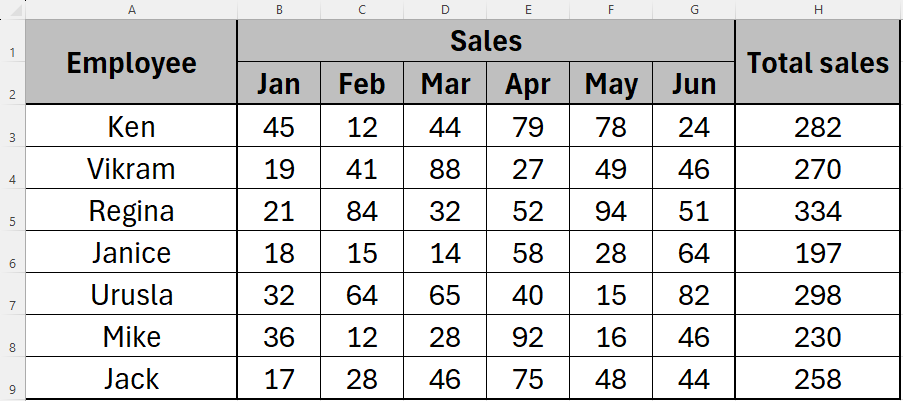
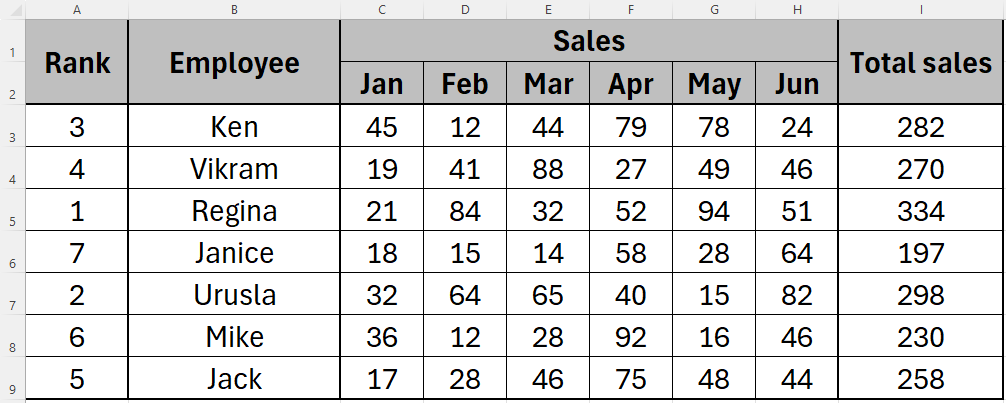
In this example, we have a list of employees and their sales data for the first six months of the year.

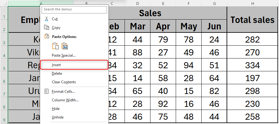
We can use the RANK function to—you guessed it—rank the employees based on their total sales. To do this, we need to create a ranking column in our existing table. If you want to later create a league table for the ranking, it’s important to place the rank at the start of your data, so the ranking column needs to be in column A. To do this, right click on the column “A” header (the part that says “A”, “B”, “C”, etc.) and click “Insert”.

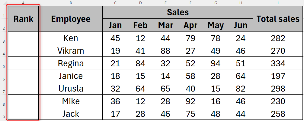
You will then see a new, blank column appear at the left-hand side of your table. Format this column as you wish and name the column “Rank”.

We’re now ready to begin our RANK formula.

Click on the first empty cell in your ranking column (in this case, A3), and type:

=RANK(

Now, click or type the cell reference of the number you want to rank (in our case, it’s I3), and add a comma:

=RANK(I3,

You now need to reference all the data you want to include in your ranking using an absolute reference, followed by a comma. In our case, that’s all the data from cells I3 to I9:

=RANK(I3,$I$3:$I$9,

Next, type “0” if you want your data to rank in descending order (that is, the highest value will be ranked first), or “1” if you want your data to rank in ascending order (with the lowest value ranked first). In our case, we want the highest value to rank first, so we will type “0”, and then close the parentheses and press Enter:

=RANK(I3,$I$3:$I$9,0)

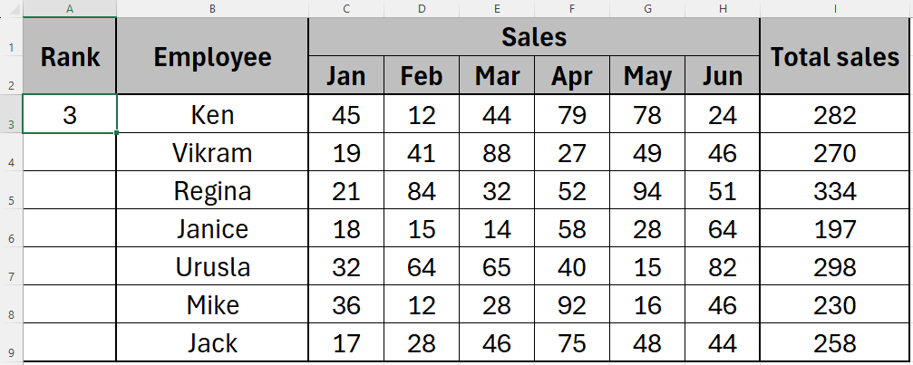
This now tells us that Ken’s total sales figure ranks third overall. Finally, use Excel’s AutoFill function to find the rankings for the remaining data in your table.

Your table now clearly tells you where each value ranks within your set of data. For tidiness, you can rename your worksheet “Totals”.

What are RANK.EQ and RANK.AVG?

RANK.EQ tells Excel to rank all equal values together, while RANK.AVG tells Excel to average the ranking for all equal values. They both follow exactly the same syntax and processes as RANK in Excel.

How to Use VLOOKUP in Excel to Create a League Table

Assuming you have already created the rankings using the method above, you can now reorder the data to produce a league table.

First, create a new sheet in your Excel workbook by clicking the “+” symbol located to the right of your tab names at the bottom of your workbook, and rename it “LeagueTable”.

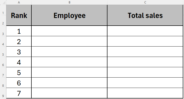
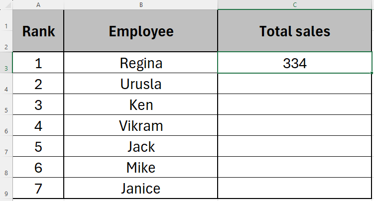
In your LeagueTable sheet, create the outline for your league table, including manually inputting the rankings into column A. In our example from the section above, we know we have seven employees to include in our league table, so we’ve typed the numbers one to seven.

We’re now ready to create the league table. The first data we want to include from our Totals sheet is the name of the employee who is ranked first. To do this, we need to use Excel’s VLOOKUP function. In cell B3, type

=VLOOKUP(

The VLOOKUP function tells Excel that you’re going to grab data from another source. In this case, we’re sourcing data from the Totals sheet in our workbook.

Next, we want to find the employee who ranks first overall, so we must reference the cell that contains the ranking “1” in our league table (in our case, that’s cell A3), followed by a comma:

=VLOOKUP(A3,

We now need to tell Excel what else it needs to consider within its VLOOKUP calculation. In this case, we want to tell it to consider all the data in the Totals table we have already created. With your cursor still blinking in the cell where you are typing the formula, go back to your Totals sheet and highlight the whole table. This will update your formula as follows:

=VLOOKUP(A3,Totals!A3:I9

Each time we apply this formula, we want the same cells in the Totals sheet to be referenced, so turn this reference into an absolute reference, and then add a comma:

=VLOOKUP(A3,Totals!$A$3:$I$9,

The penultimate part of this formula is to tell Excel where to look to find the detail we want to insert into the cell we’re typing in. In this example, we want to see the name of the person who ranks first.

In our Totals table, there are nine columns overall, and the names of the employees are in the second column of that table, so we type the number two, followed by a final comma:

=VLOOKUP(A3,Totals!$A$3:$I$9,2

And finally, type “FALSE” to tell Excel to find an exact match, before closing your parentheses and pressing Enter:

=VLOOKUP(A3,Totals!$A$3:$I$9,2,FALSE)

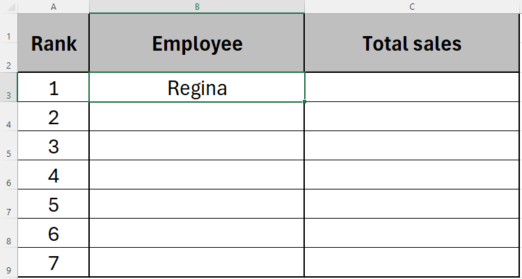
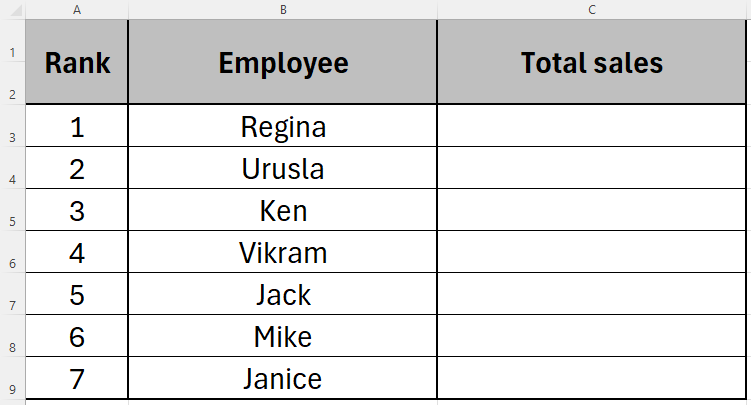
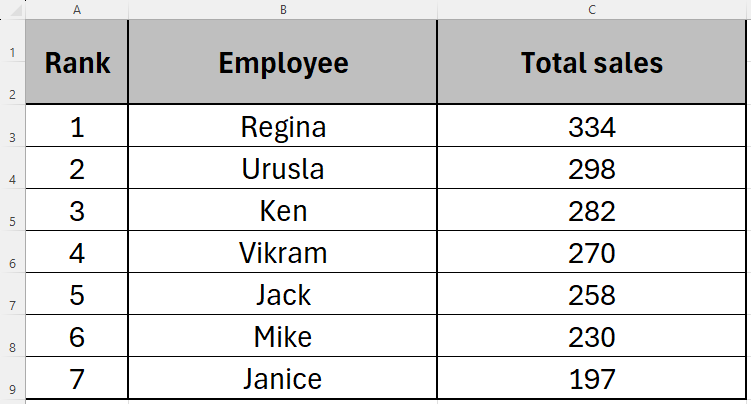
This now tells us that Regina is the highest-ranked employee. Use Excel’s AutoFill function to complete the rest of the employees’ names.

Now that we can see the employees in order based on their total sales from the Totals sheet, we can add their total sales using VLOOKUP in the same way.

This would be the formula we place in cell C3:

=VLOOKUP(A3,Totals!$A$3:$I$9,9,FALSE)

Notice that this time, we have input “9” as the penultimate part of our formula, as we want Excel to capture the total sales from the ninth column in our Totals table.

Complete the table by using AutoFill down column C.

If you were to change the data in your Totals sheet, the league table would automatically update to reflect the changes.

That’s it! You now have all the tools you need to use the RANK function in Excel, and combine this with VLOOKUP to create a league table. If you do indeed choose to add the league table to your workbook, after you have done this, you can tidy up your original Totals sheet by hiding the column containing the rankings.