Excel’s TAKE function will let you extract the first, last, or specific columns or rows from a table. For example, you might want to extract the data from the last three days or display the top ranked individuals. Let’s look into this in more detail.
Excel’s TAKE function only works in Microsoft 365 or Excel for the web.
Prepare Your Table in Excel
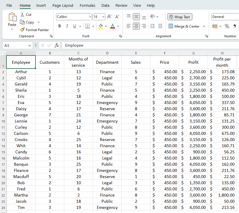
Before you can use TAKE and CHOOSE, you will need to format and name your table. We will use this table of data as our example:
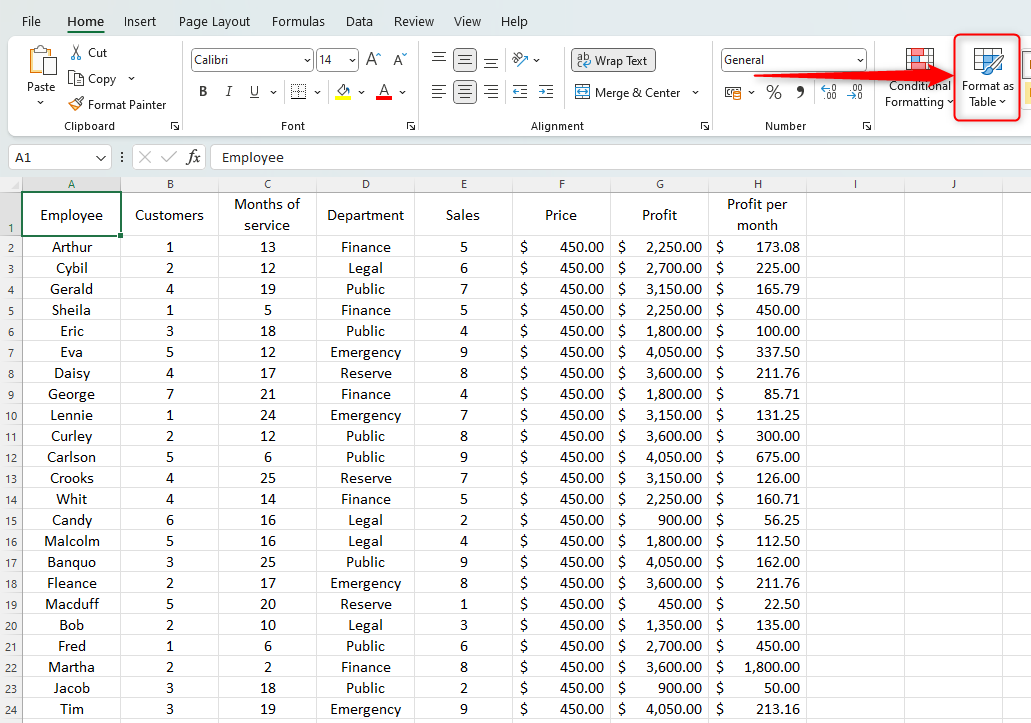
Ensure you have included a row that includes headings for your columns. Now, select any cell within your table and click “Format As Table” in the “Styles” group of the “Home” tab.
Click your preferred layout and, in the dialog box that opens, check “My Table Has Headers” and click “OK”.
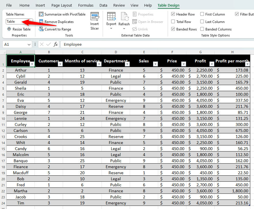
Now that Excel recognizes your data as a formatted table, you need to change the table name (for later use). In the “Table Design” tab on the ribbon, head to the “Properties” group and change the “Table Name” field to one that works for you.
You’re now ready to extract data.
How to Use TAKE to Extract the First and/or Last Rows and/or Columns in Excel
Excel’s TAKE function is mostly used to extract the first or last few rows or columns from your table. The formula you’ll need to use is:
=TAKE(X,Y,Z)
where X is the table name, Y is the number of rows to extract, and Z is the number of columns to extract. Simply place a “-” in front of Y or Z to change that part of the formula from the first rows or columns to the last rows or columns.
If the number of rows or columns that you want to extract might change, instead of typing digits for Y and Z, you can place the number in another cell and type the appropriate cell reference.
In our example, we want to find out the names of the top five employees based on profit per month.
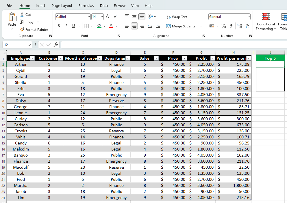
First, create a place on your worksheet where you want the data to be extracted, and type an appropriate header. In our case, we’ve chosen cell J2 and the header “Top 5.”
Second, start to type the formula as follows:
=TAKE(
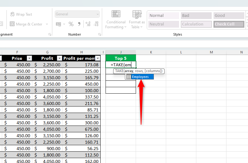
The next part of your formula is the table name. Begin typing the name of your table in your formula, and then double-click when you see it appear in the suggestions box. Then, add a comma.
=TAKE(Employees,
You now need to tell Excel how many of the first or last rows you want to include in your extracted data. In our case, we want the top five employees. Therefore, we type “5” and add a comma. If we wanted the last five rows, we’d type “-5”. To extract all rows, simply don’t include the number, and add the comma.
=TAKE(Employees,5,
Finally, finish your formula by telling Excel how many of the first or last columns you want to include. We’ll go for just the first column, as we want only the employees’ names, and close the parentheses and press Enter. Again, type “-” if you want to extract the last x columns. To extract all columns, miss out the number and press Enter.
=TAKE(Employees,5,1)
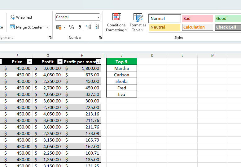
You will now see the desired outcome. Now, if you change or reorder the data in your table, the TAKE formula you have just added will automatically adjust to extract the updated information. For example, we want to reorder the column containing profit per month:
If you were to add more data to your table, the TAKE formula would account for this. For example, if we added another employee’s data to the bottom of the table in an additional row (by dragging the corner handle of the table downwards one row and completing their figures), the TAKE formula would include this when looking for the criteria you set.
How to Use TAKE to Extract a Specific Column in Excel
If you want to extract a specific column, follow the steps above but add the column name to your formula in place of the number of columns.
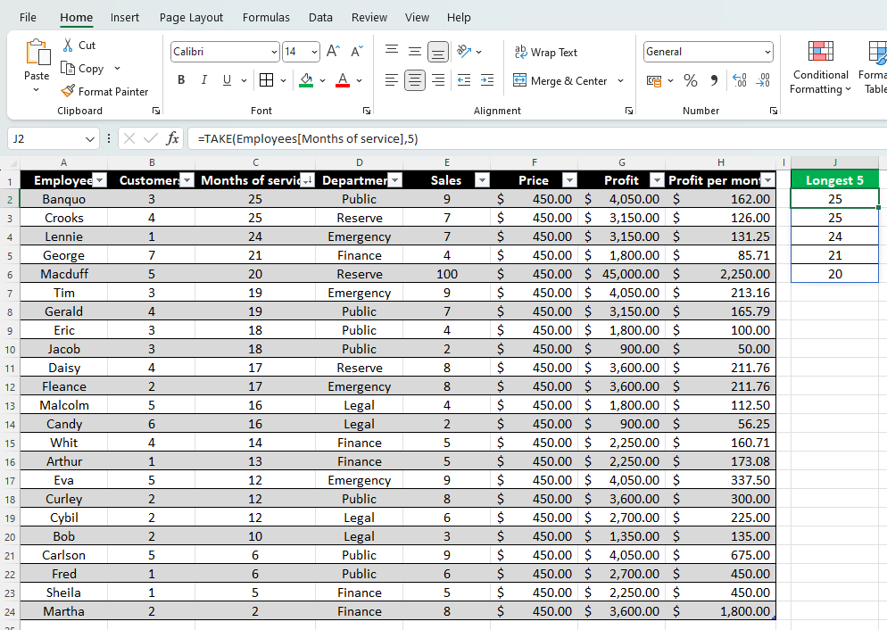
Let’s say that, in our example above, we need to work out how many months each of the five longest serving employees have been at the company. This would be our formula:
=TAKE(Employees[Months of service],5)
where “Employees” is the table’s name, “[Months of service]” is the column name (notice the lack of a comma in between these two parts of the formula), and “5” is the number of rows we want to extract from the named column. Remember to filter the corresponding column in your table.
How to Use TAKE with AVERAGE in Excel
If you want to use TAKE with Excel’s AVERAGE function, follow the steps above but nest the TAKE formula within your AVERAGE formula.
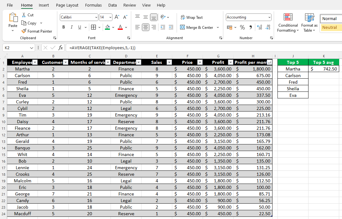
For example, let’s say we want to work out the average earnings of the top five employees. This would be our formula:
=AVERAGE(TAKE(Employees,5,-1))
where the AVERAGE formula surrounds the TAKE formula, which includes “Employees” (table name), “5” (we want to take the top 5 rows), and “-1” (we want to take the last column).
You now have a fundamental understanding of how the TAKE formula works in Excel. You can now go one step further—extract columns or rows from multiple ranges by using Excel’s VSTACK and HSTACK functions, or combine TAKE with Excel’s SORTBY function to see it work without you sorting your table’s columns. Finally, you can use Excel’s DROP function, which excludes certain cells and rows from your extracted data and works with exactly the same syntax as the TAKE function.
source
