If you have data across multiple Excel worksheets that you want to bring together in a formula, don’t waste time manually referencing each cell. Instead, use an Excel function called 3D referencing, which helps speed up the process and ensure you don’t accidentally exclude any cells.

Why Referencing Manually in Excel Can Cause Problems

The beauty of using 3D referencing is that it can help you to avoid potential pitfalls versus manually selecting cells across worksheets one by one. For example, if referencing manually, you might accidentally miss the relevant cell in one of your worksheets, or you might reference an incorrect cell. Furthermore, if you have many worksheets, manually working across them is cumbersome and time-consuming.

While 3D referencing isn’t flawless, which we’ll touch upon later, it is a way to navigate these potential issues and ensure both accuracy and efficiency.

How to Use 3D Referencing in Excel

Here are the steps to follow to use 3D referencing in any version of Excel.

Step 1: Lay Out Every Worksheet the Same Way

For 3D referencing to work, you need to make sure each worksheet you are referencing is laid out the same way—or, at least, the cell you need to capture in your formula is the same cell in each worksheet.

As you can see here, across the two worksheets “January” and “February”, each person’s totals are in the same cell (Sarah’s are in B2, John’s are in B3, and so on).

Step 2: Add a Start Sheet and an End Sheet

The next step is to add a start sheet and an end sheet to your workbook. These act as bookends, and we’re going to create a formula to capture anything between them. This means that if you add new worksheets and want them included in your referencing, you should place them between these bookends.

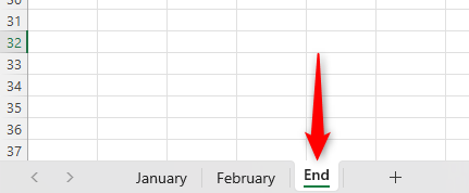
First, add an end sheet. To do this, click the final tab in your workbook and then select “+” to add a new worksheet. You can then rename the new worksheet to “End” by double-clicking on the worksheet name in the tabs.

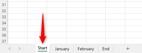
Now, you need to add a start sheet to your workbook. Again, select “+” to add a new worksheet, and rename this to “Start”. Then, click and drag your “Start” sheet to the left of all existing tabs.

Step 3: Add a Totals Sheet

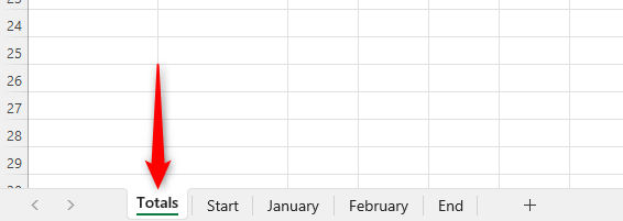
If you haven’t done so already, add a worksheet to place the formula’s output. Once again, click “+”, rename the new worksheet to “Totals”, and then click and drag this new sheet to the left of all existing tabs to place it at the start of your workbook.

Step 4: Create the Formula in the Totals Worksheet

We are now ready to begin the 3D referencing. Using the example above, let’s say we want to find out Sarah’s total earnings for January and February combined. Sarah’s monthly totals are in cell B2, so we want to add together the value in cell B2 from each worksheet.

In the “Totals” worksheet, click the cell where you want Sarah’s yearly total to be calculated. In that cell, type the following:

=SUM(

Next, click the “Start” worksheet, hold Shift on your keyboard, and click the “End” worksheet. Then click the cell you want to reference (in the example above, that’s cell B2). Finally, type a close bracket and press Enter. You will see the following formula appear in the formula bar at the top:

=SUM(Start:End!B2)

This will now pick up cell B2 for “January”, “February”, and any other worksheet you add between the “Start” and “End” worksheets.

Remember, if you add a new worksheet, make sure you place it somewhere between the “Start” and “End” worksheets, and use the same layout.

If your “Totals” worksheet has the same layout as your individual data worksheets, you can use Excel’s Autofill function to avoid retyping the formula for each calculation. Alternatively, you can press Ctrl+C on the cell with the formula, and then press Ctrl+V on the other cells where you want the same function to occur.

Using 3D Referencing Across a Range of Cells

To use 3D referencing across a range of cells, follow the same steps as above. However, rather than clicking on a single cell when creating your formula (in the previous example, this was cell B2), highlight all the cells you want to include in the calculation.

In this example, it would be B2, C2, D2, and E2. This will pick up the total for all four values on each worksheet:

=SUM(Start:End!B2:E2)

If the cells you want to reference are not adjacent to each other, hold Ctrl on your keyboard and then click all the cells you want to capture in the formula. In this example, it will pick up cells E7, R16, and M24 on each sheet:

=SUM(Start:End!E7,Start:End!R16,Start:End!M24)

Potential Issues With 3D Referencing

As with all Excel functions, there are some potential pitfalls you need to watch out for when using 3D referencing:

• If you add a new worksheet after the “End” worksheet or before the “Start” worksheet, your formula will not capture these new worksheets. Make sure you always position new worksheets between your bookends.
• If you adjust a workbook’s layout (like adding a new row or column), the inconsistency in layouts between your worksheets will cause formula miscalculations because the wrong cells will be referenced. Make sure you always maintain the same layout across all referenced worksheets.
• If you hide a worksheet, even though you cannot see the data it contains, the formula will still pick the data up. Make sure you are aware of this when looking at your totals.
• If you delete a worksheet that is referenced within your formula, the data from this worksheet will automatically be discounted from your calculations.

That’s it! You now know how to save time through 3D referencing and be confident that your cross-worksheet referencing is accurate and dynamic.